Summary by Kellee Mundy
Master of Accountancy Program
University of South Florida, Summer 2003
Deming Main Page |
Quality Related Main Page
This article discusses the importance of measuring hidden quality costs that are associated with a product. Quality costs are defined as “costs incurred for ensuring conformance to quality standards or compensating for nonconformance to quality standards” (page 8). Conventional accounting systems are not able to measure intangible quality costs, so these costs become hidden quality costs. Some examples of hidden quality costs are customer dissatisfaction with a product or defects in a product that causes a loss in sales. These hidden quality costs can be the major factor in the total cost of quality for a product.
Taguchi’s Quality Loss Function
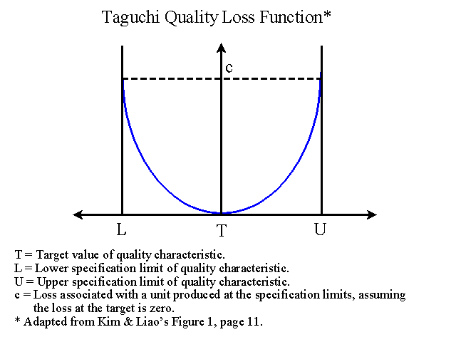
To estimate these hidden quality costs, a Taguchi quality loss function (QLF) has been proposed. Taguchi’s approach is different than the traditional approach of quality costs. In the traditional approach, if you have two products and one is within the specified limits and the other is just outside of the specified limits, the difference is small. Although the difference is small the product within the limits is considered a good product while the outside one is considered a bad product. Taguchi disagrees with this approach. Taguchi believes that when a product moves from its target value, that move causes a loss no matter if the move falls inside or outside the specified limits. For this reason, Taguchi developed the QLF to measure the loss associated with hidden quality costs. This loss happens when a variation causes the product to move away from its target value.
The QLF is a “U” shaped parabola. The horizontal axis is tangent with the parabola at the target value. This is a quadratic loss function because it assumes that when a product is at its target value (T) the loss is zero.

The unit loss is determined by the formula:
L(y) =k(y-T)2
Where:
k = a
proportionality constant dependent upon the organization’s failure cost structure,
y = actual value of quality characteristic,
T = target value of quality characteristic.
The value of k must first be determined before the loss can be estimated.
To determine the value of k:
k= c/d2
Where:
c = loss associated with the specification limit, and
d = deviation of the specification from the target value.
The value of k determines the slope of the QLF, the larger the value of k the steeper the parabola. This is a symmetric QLF because it is assumed that there is a constant k for the whole loss function. The value of c is a major component in the loss function. This value represents the intangible quality costs of a product.
Asymmetric Quality Loss Function
The term asymmetric implies that variations can have different sensitivities to loss. If a variation happens on one side of the loss function, that loss may be more or less sensitive than if the same amount of variation happened on the other side of the target value. This involves having to add to the previous formula, there will now be two k’s. k will now represent the different sensitivities that happen when a variation moves on either side of the target value. This loss function now becomes an asymmetric QLF because there can be different values for k.
The unit loss function becomes:
L(y) = k1[(y-T)+]2 + k2[(T-y)+]2
Where: k1 > or < k2
x+ = Max (x,0)
Again k must be determined before the loss can be estimated.
k1 = c1 / (U-T)2
k2 = c2 / (U-T)2
Where: U = upper specification limit of characteristic,
L = lower specification limit of characteristic,
c1= loss associated with U, and
c2 = loss associated with L.
Example Using the Asymmetric Quality Loss Function
Given these values:
c1 = $80, c2 = $48, U = 10.4mm, L = 9.6mm, and T = 10mm
First the value of k must be determined.
k1= 80 / (10.4-10)2 = $500
k2= 48 / (10-9.6)2 = $300
Now the estimation of loss can be determined. Assume that a variation of .2mm happened on both sides of the target value. The product with an actual value of 10.2mm, moved to the right of the target value
L(y =10.2) = $500(10.2 -10)2 + $300(0)2 = $20
Or actual value of 9.8mm, moved to the left of the target value
L(y =9.8) = $500(0)2 + $300(10-9.8)2 = $12
Since c1 > c2, then k1 > k2. This implies that the right side of the loss function is more sensitive than the left side. In the example above the product moved .2mm in both directions and the move to the right causes the greater loss.
Insensitive Region of Quality Loss Function
This deals with different levels of loss sensitivity on either side of the target value. Insensitive means that there could be different sections in the loss function that are more or less sensitive than other sections. These sensitivity differences cause larger losses in some sections in relation to other sections of the loss function. For these situations, a separate L(y) formula is needed for each different section in the loss function.
Examples
| Case | Product, service or characteristic | Effect or explanation |
| Symmetric with insensitive regions. | Soft drinks, juice and medicine. | A small deviation from the target value does not create a significant loss, but is not negligible. But too much or too little of an ingredient can cause a large loss. |
| Asymmetric with insensitive regions. | Product delivery time and customer service. | Early delivery causes small loss, but late delivery causes larger loss. |
| Asymmetric with insensitive regions. | Air pressure in auto tires. | Too little air may cause some loss in performance, but too much air can cause a large loss from a blow out. |
| Asymmetric with zero loss in insensitive regions. | Blood pressure and blood cell count. | Within a range of variation from the target there is no loss. Any further deviation from the target value may cause significant loss. |
Summary
Many of the quality costs associated with a product are not recorded. Therefore, estimates need to be made of these hidden quality costs. Estimates of hidden quality costs are needed so that managers can understand and control those hidden costs. “Quality loss functions provide a vehicle for reasonable estimates and meaningful understandings of hidden quality costs, which are necessary for effective control of product quality costs” (p. 17).________________________________________________
Related summaries:
Albright, T. L. and H. Roth. 1992. The measurement of quality costs: An alternative paradigm. Accounting Horizons (June): 15-27. (Summary).
Albright, T. L. and H. P. Roth. 1994. Managing quality through the quality loss function. Journal of Cost Management (Winter): 20-37. (Summary).
Anderson, S. W. and K. Sedatole. 1998. Designing quality into products: The use of accounting data in new product development. Accounting Horizons (September): 213-233. (Summary).
Deming, W. E. 1993. The New Economics for Industry For Industry, Government & Education. Cambridge: Massachusetts Institute of Technology Center for Advanced Engineering Study. Chapter 10. (Summary).
Joiner, G. L. and M. A. Gaudard. 1990. Variation, management, and W. Edwards Deming. Quality Progress (December): 29-37. (Note).
Martin, J. R. Not dated. Chapter 3: Cost Behavior Analysis & Statistical Process Control - Part II. Management Accounting: Concepts, Techniques & Controversial Issues. Management And Accounting Web. Chapter3PartII.htm
Martin, J. R. Not dated. Constrained optimization techniques. Management And Accounting Web. ConstrainoptTechs.htm
Martin, J. R. Not dated. Summary of the 1992 PBS Program Quality or Else. Management And Accounting Web. QualityOrElse.htm
Martin, J. R. Not dated. What is Six Sigma? Management And Accounting Web. SixSigmaSummary.htm
Roth, H. P. and T. L. Albright. 1994. What are the costs of variability? Management Accounting (June): 51- 55. (Summary).
Sedatole, K. L. 2003. The effect of measurement alternatives on a nonfinancial quality measure's forward-looking properties. The Accounting Review (April): 555-580. (Summary).
Shank, J. K. and V. Govindarajan. 1994. Measuring the "cost of quality": A strategic cost management perspective. Journal of Cost Management (Summer): 5-17. (Summary).
Taguchi, G. and D. Clausing. 1990. Robust quality. Harvard Business Review (January-February): 67-75. (Summary).